Probably this will be a fast introduction to the some ideas in deep learning called SFT (Supervised Fine Tuning). After pre-training a language model, for better reasoning (or task completion) in precise topics fine-tuning is a must for full training of the language model.
LoRA - Low Rank Adaptation
A pre-trained autoregressive language model denoted by $$P_\phi(y\lvert x)$$ parametrized by set of parameters $\phi$. One can understand the task of a language model with these examples better:
| $x_i, y_i$ | Task 1 | Task 2 |
|---|---|---|
| $x_i$ | Content | Natural Language |
| $y_i$ | Summary | SQL |
Remember that both $x_i$ and $y_i$ are tokens. Each task has some type of training dataset $Z=\lbrace(x_i,y_i)\rbrace_{i=1,\dots,N}$.
Full Fine-Tuning
Let $\phi_0$ be pre-trained weights of the model (after the pre-training), again like many of the tasks in deep learning this is a gradient descent too:
$$\phi_0+\Delta \phi$$
Again by mere backpropagation over whole parameter set one can fine-tune the model via this basic descent. This gives us a maximization problem for finding the maximizer parameter $\phi$:
$$\argmax_{\phi}\sum_{(x,y)\in Z}\sum_{t=1}^{\lvert y \rvert} \log{(P_\phi(y_t | x, y_ {<t}))}$$
From this maximization we can easily see that each tuning step learns different set of $$\Delta \phi$$ which has dimension $\lvert \Delta \phi \rvert = \lvert \phi_0 \rvert$. One can think that we already trained (pre) this many parameters but we actually got a heavier problem than normal pre-training: if we use the whole parameter space for training we are using it that many parameters for whole steps of fine-tuning. One great example is directly the example given in the LoRA paper: GPT-3. GPT-3 is a direct transformer model with 175 billion parameters, so for every step of full fine-tuning you need to load whole set of 175 billion parameters for the backpropagation updates. So, clearly it is awful. We actually have some more appropriate ways to fine-tune a model but today we are going to talk about one of the most important methods in low-rank fine-tuning.
A More “Parameter-Efficient” Approach
From now on we do not need to use the whole parameter set to introduce weight updates to the backpropagation. Some “intrinsic rank” property of training matrices directly allows us to use some part of the parameter space as:
$$\Delta \phi = \Delta \phi(\Theta),$$
where $\Theta$ is a smaller sized set of parameters. For a meaningful increase in performance (and intrinsic rank allows us again) we must choose the size of our new smaller parameter set as:
$$\lvert \Theta \rvert « \lvert \phi_0\rvert$$
Thus task of finding the new update parameters $\Delta \phi$ becomes
$$\argmax_{\Theta}\sum_{(x,y)\in Z}\sum_{t=1}^{\lvert y \rvert} \log{(P_{\phi^*}(y_t\lvert x, y_ {<t}))},$$
where $\phi^*=\phi_0+\Delta\phi(\Theta)$.
Up to here everything is still abstract. We said “take a much smaller set $\Theta$ and encode $\Delta\phi$ with it”, but we never said how one should choose this $\Theta$. The whole content of the method is hidden in that choice, so let us make it concrete.
Low-Rank Parametrized Update Matrices
The starting point is an observation of Aghajanyan et al.: a pre-trained language model has a low intrinsic dimension, meaning you can randomly project its parameters into a much smaller subspace and it still learns efficiently. LoRA takes one step further and makes the hypothesis not about the parameters but about the updates: if the model itself already lives on a low dimensional subspace, then the change we apply to it during adaptation should also have a low intrinsic rank.
So instead of the whole parameter set, look at a single dense layer with pre-trained weight matrix
$$W_0 \in \mathbb{R}^{d\times k}$$
and constrain its update by a rank decomposition
$$W_0 + \Delta W = W_0 + BA, \quad B\in\mathbb{R}^{d\times r},\ A\in\mathbb{R}^{r\times k},\ r « \min(d,k).$$
Here $W_0$ is frozen, it receives no gradient at all, and only $A$ and $B$ are trainable. Note that $W_0$ and $\Delta W = BA$ are multiplied with the same input and their outputs are summed coordinate-wise, so for $h=W_0x$ the modified forward pass is simply
$$h = W_0x + \Delta W x = W_0 x + BAx.$$
Counting parameters, we went from $dk$ to $r(d+k)$ for that layer, and since $r$ is tiny (the paper uses $r=1,2,4,8$ while $d$ can be $12{,}288$) this is exactly the $\lvert\Theta\rvert « \lvert\phi_0\rvert$ we asked for above.
Two small but important details about how this is set up:
- Initialization. $A$ is initialized with a random Gaussian and $B$ is initialized to zero, so $\Delta W = BA = 0$ at the beginning of training. This means you start exactly from the pre-trained model, you do not perturb a perfectly good model with random noise before the first step.
- Scaling. $\Delta W x$ is scaled by $\frac{\alpha}{r}$, where $\alpha$ is a constant in $r$. When you optimize with Adam, tuning $\alpha$ is roughly the same thing as tuning the learning rate, so the authors just set $\alpha$ to the first $r$ they try and never tune it again. The point of the scaling is that you do not have to retune your hyperparameters every time you change $r$.
A Generalization of Full Fine-Tuning
This is the part I like most. A more general form of fine-tuning already allows you to train only a subset of the pre-trained parameters, and LoRA goes further: it does not force the accumulated update to be full rank. But the direction also works backwards. If you apply LoRA to all weight matrices and let the rank $r$ grow up to the rank of the pre-trained matrices, you roughly recover the expressiveness of full fine-tuning. In other words, as the number of trainable parameters increases, training LoRA converges to training the original model.
Compare this with the alternatives and the picture becomes clearer: adapter-based methods converge to an MLP as you grow them, and prefix-based methods converge to a model that cannot take long input sequences. LoRA is the only one of the three whose limit is the thing we actually wanted in the first place.
No Additional Inference Latency
At deployment you can explicitly compute and store
$$W = W_0 + BA$$
and then run inference exactly as usual. Both $W_0$ and $BA$ live in $\mathbb{R}^{d\times k}$, so nothing about the shape of the network changes and there is no extra latency, by construction. Switching to another downstream task is just subtracting $BA$ and adding a different $B’A’$, which is a cheap operation with very little memory overhead. This is precisely what adapter layers cannot do, because they sit in series with the base model and therefore must always be computed on top of it.
The Picture Behind All of This
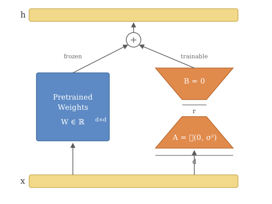
Everything we did above is in this one diagram, and it is worth reading it slowly.
The input $x$ enters at the bottom and immediately splits into two parallel paths. The left path is the frozen highway: it goes through the pre-trained $W$ and comes out as $W_0x$, untouched, exactly as it was before we started fine-tuning. The right path is the detour we are actually training.
Look at the shape of that detour. The lower trapezoid $A$ starts wide (dimension $d$) and narrows to $r$; the upper trapezoid $B$ starts at $r$ and widens back to $d$. That pinch in the middle is the whole method drawn as a picture. Whatever the detour wants to say about the input, it must first be squeezed through $r$ dimensions before it is allowed to expand back. The rank constraint is not an extra condition we impose afterwards, it is the geometry of the branch itself.
The colors carry the second half of the story. Blue is frozen, orange is trainable, and only the orange parts get gradients or optimizer states. This is where the memory saving comes from: for a large transformer trained with Adam you do not have to keep the optimizer states for the frozen parameters at all.
The labels inside the trapezoids are the initialization we mentioned: $B=0$ and $A=\mathcal{N}(0,\sigma^2)$. Read together with the diagram this says that at step zero the right path multiplies everything by zero, so the sum at the top is just $W_0x$ and the model is the pre-trained model. Note also that we cannot set both to zero, because then no gradient would flow through either matrix and the branch would be dead forever; one of them being Gaussian is what keeps the thing alive.
Finally, the $+$ at the top. The two paths are summed coordinate-wise, not composed, and both branches are linear in $x$. This is the reason $W_0x + BAx = (W_0+BA)x$, which is exactly why you can fold the orange part into the blue one at deployment and pay nothing at inference time. If the detour were placed after the blue box instead of beside it, as in adapters, no such folding would exist and you would carry the extra depth forever.
So the picture is really the argument: parallel instead of sequential gives you the free merge, the bottleneck gives you the parameter efficiency, and the zero initialization gives you a safe starting point. In the next part we can look at what happens when you actually ask which weight matrices deserve this treatment, and how small $r$ is allowed to get before the whole thing breaks.